


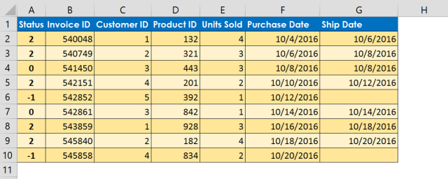
Imagine we have a spreadsheet that records a purchase date for when your customer places an order and a ship date for when the product ships. We would like to have a red flag in column A for orders that currently have not been shipped. And if the product has shipped we would like a green check mark. See the below the example and then keep reading and I’ll show you how to create this spreadsheet using either Excel 2007, 2010, 2013 or 2016. Note that row 6 and row 10 displays a red flag because those orders have not been shipped.

Step 1: Click in cell A2 and write a formula =IF(G2=””,-1,G2-F2). This IF function checks if the Ship Date is blank. Excel an verify if there is a blank cell by using the formula =”” so if G2=”” is true then make the value equal to -1. Otherwise, if the ship date is not blank, then use the formula to equal ship date minus purchase date [G2-F2]. The answer will be zero if the order has the same ship date as the purchase date. Note that on row 4 and row 7 that the formula equals zero because the ship date is equal to the purchase date which results in 0.
Step 2: Copy the formula down using the auto fill handle.
Step 3: With the status cells selected in column A, choose the Conditional Formatting command from the Home tab. Select the icon sets menu and then click the 3 symbols (Uncircled).
![]()
Step 4: Click Conditional Formatting –> manage rules –> Edit formatting rule.
Step 5: Click show icon only (Screen shot below is from Excel 2013. Will look a little different in Excel 2007)
Step 6: Green check mark icon when value is >=0 Number. (Replace percent with number from the type drown down). Type a zero in the value area.
Step 7: Click no cell icon for when < 0 and >=0 Number. ( the middle range yellow exclamation mark will be replaced with no cell icon.
Step 8: Change the red X with a red flag for when <0 and click OK.


Hello Steve,
I am totally new to this so please bear with me. I have what is probably to you a simple need but one which is driving me up the wall.
I want to use Green Amber Red to show an action status.
My need;
The action has a start date (e.g. in A1) and a completion date (e.g. in B1). When a start date is entered in A1 and a completion date (which is for fixed periods of 6 months, 12 months or 18 months), is entered in B1, in C1 a green icon appears (I would like this column blank until dates are entered). 30 days before the due date icon turns amber, on due date icon turns red.
Any help you could provide would be much appreciated.
This is something I started but needs a little bit more work. The challenging issue is that you have a moving target with the =today(). https://1drv.ms/x/s!AmOflzuTYrYwmZRh8Pjlcc5cris_gA
Dear Steve,
Thanks for taking the time to do this, I have had a play and it seems exactly what I need. As said previously, you need to bear with me. I can see and understand the formula in column ‘C’ and the conditional formatting rules which I can adapt for my spreadsheet, Can I just clarify that the extra bit of wording in G/H 2, 3, 4 is some welcome additional explanation. I cannot see that it has any active part in your work.
You also say that it needs a little more toil, I would be interested to know what more you could be doing to improve this.
Once again many thanks
RayG
The extra bit of wording was just some notes for me to look at while I preparing the spreadsheet. They have no impact on the formatting or formulas. The problem that I thought of that needs more work is that I used the TODAY() function which is dynamic to today’s value. So that would create red x’s to appear when for anything in the past. I’m thinking that if the completion date is in the past then there should be a green check, correct? Do you always want a green check to display when it is completed even if it is late?
Steve,
You have hit on something I hadn’t even thought of. Of course there should and will be occasions when the project completes on time, which means green should be the indicator. If I have it right at the moment all entries will end with a red indicator no matter if completed in time or not. I’m thinking this is going to need a manual intervention, would I be able to over ride the formatting in a particular cell to reflect the final status?
RayG
Yes, you are on the right track. One of the powers of Conditional formatting is the “Stop when true” feature when you have multiple conditions. When you click manage rule all the rule will sequence in the order top down. You can arrange them so that the first one is a statement to something that tests the TODAY() to the project end date.