


I want to use the data set to lookup the items associated by month.
At any given month, I want to lookup the values for the revenue and expenses per ID. The IDs are listed above but they are located in merge cells. This creates a problem because typically tables do not have merge cells. But with using the index and match function I can lookup the data I want.
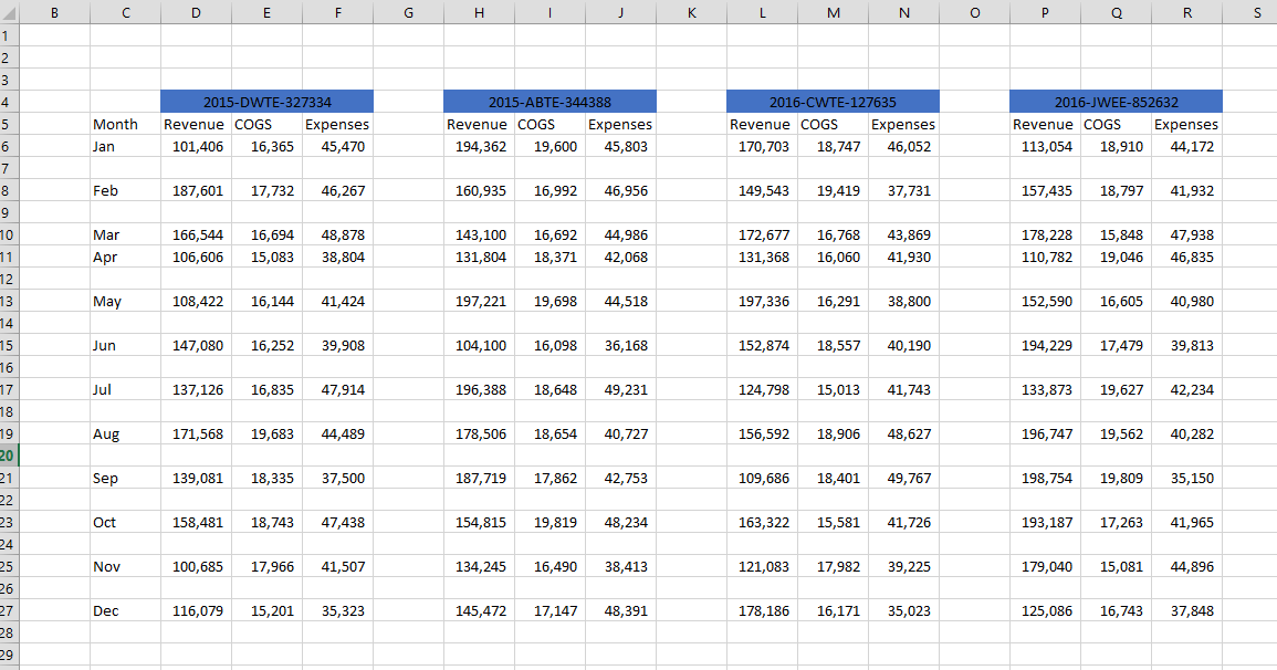
I will need to create 3 range names. One for the data range, one for the horizontal labels, and the other for the vertical labels.
The index function has 3 arguments. First I use the data range, then I need a row number to go down and the column number to go across to the right. So if I did =index(DataRange,1,1) I would return the top left most cell of the range which in the graphic above is 101,406.
Better to use the match function that can return a number to go down to the certain row and again to the column number to the right.
For example =match(“Jan”,MonthRange,0) would return 1 assuming that Jan because Jan is the first row of the range.
In the video I use this function =INDEX(DataRange,MATCH(U$8,MonthRange,0),MATCH(T10,IDRange,0)) where U$8=”Jan” and T10 =”2015-DWTE-327334″.
Download my printable Excel Keyboard Shortcuts.
Practice with a index and match sample I used in the video tutorial.


Leave A Comment